
Loading radar observations quickly is only part of preparing them for machine learning. Radar volumes contain sweeps with different elevations, timing, and sampling patterns. How should we organize those observations into training samples?
In our collaboration with NOAA on compact radar representations, we developed Raystacks: a representation that assembles radar observations across sweep and volume boundaries. Our introduction to radrs covers the reader and its loading performance; here we explain how the representation supports model training.
Raystacks: AI-ready ray data
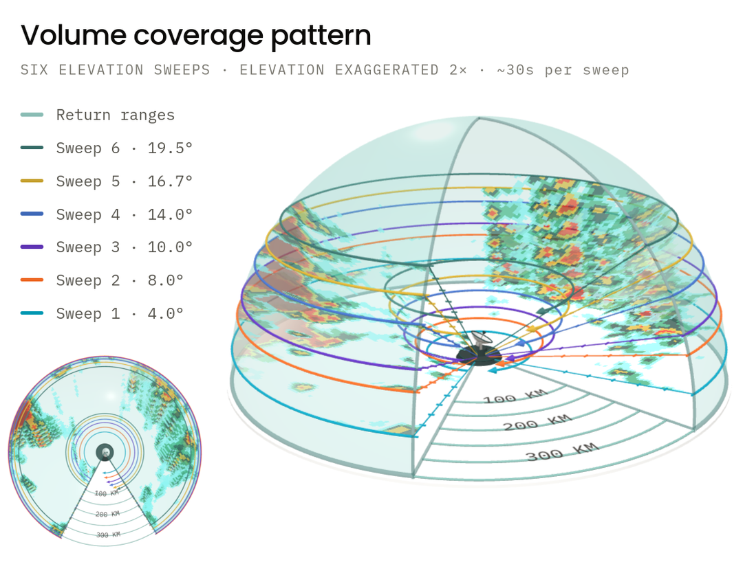
Early on in our NOAA collaboration into compact radar representations, a key encoding question was apparent. Radar systems such as NEXRAD achieve 3D observations through dynamic and changing "volume coverage patterns" (VCPs), where the radar aperture can be swept across the 3D FOV in a combinatorial number of trajectories. These are often organized in the form of "sweeps" at different angles for rotating systems.
Different VCPs with different sweep strategies represent different observational tradeoffs. For example, VCP-35 consists of long-range data collected on clear days while VCP-215 is used to get finer, closer structure of an ongoing storm. In addition, sweep-level variants can be executed to capture different types of return data or differential sweep information. Many radar platforms are also mobile themselves, allowing observations of the same storms from multiple locations.
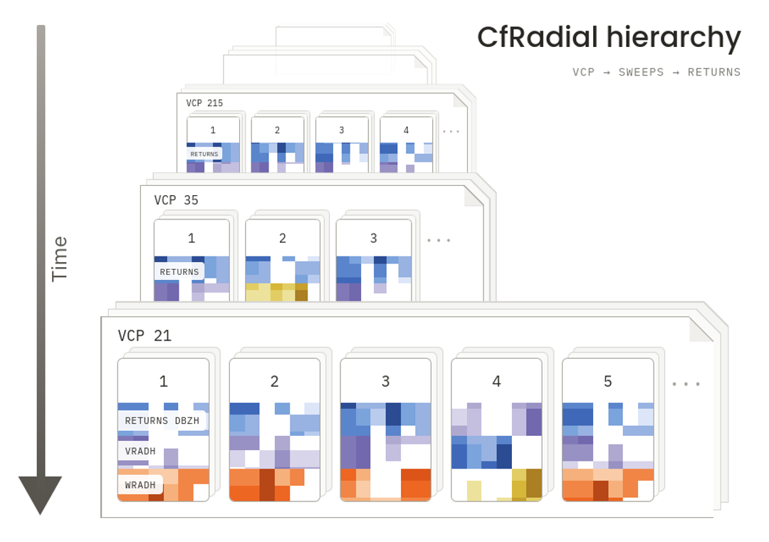
The current standard of data collection for radar returns, CfRadial (supported by the excellent XRadar library in Python) captures all this information in a compact, but nested and irregular way. Each VCP stands alone as a tree of data with variable number of sweep branches, each of which may have irregular return cadences. This makes the format challenging to ingest as a modeling input, but just as importantly implicitly hardcodes assumptions about radar timing and sweep relationships that might be otherwise generalized by AI.
The Raystack data structure was our solution to this problem. In a Raystack, the complex hierarchy of returns is flattened into a single stream of "rays" per variable over time. There are no built-in constraints over ray positions or cadence in spacetime - single, multiple, or moving apertures are supported. This makes batching and windowing particularly simple - ray data can be aggregated into VCP sub- or supersets without design changes.
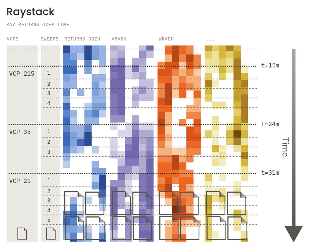
Sweep and VCP metadata remain represented in Raystacks, but as sibling metadata channels of data. These streams of sweep and VCP "timestamps" are produced alongside the stream of returns, allowing (but not requiring) models to integrate the additional context. Future coverage patterns might produce different meta streams (perhaps from phased array systems), but importantly would retain the same Raystack structure supporting generic storage and correlation.
What a model receives
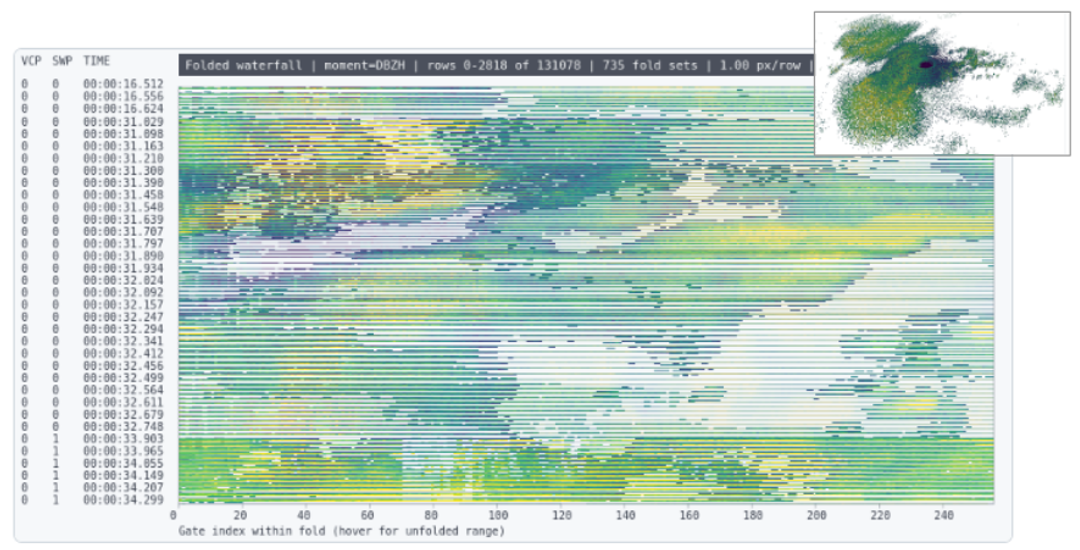
In radrs, a return is a fixed-width chunk of range gates from one physical ray. The fold_size setting controls the width. For example, a ray with 1,832 gates and fold_size=128 becomes 15 return rows: 14 full chunks and a final chunk with 40 observed gate positions followed by padding. This partitioning is what we call folding.
Each radar variable is a matrix shaped (n_returns, fold_size). Time, azimuth, elevation, base range, and range step align with its rows. The range coordinate is an index within the chunk: physical distance is base_range + gate_index × range_step. Sweep and VCP tables retain the scan context, and each sweep’s num_returns records how many rows belong to it. Apply the same row selection to the observations and their metadata when assembling a sample.
Building dense training samples
For a training sample spanning consecutive scans, BatchedRaystack appends observations from multiple volumes into shared arrays. Concurrent fetching can overlap network reads with parsing. We can then select return rows within a time window across sweep and volume boundaries, keeping their time and spatial metadata alongside the observations.
Batching still requires a completeness check: reserve enough capacity and verify how many volumes were added, since capacity limits or fetch failures can leave gaps. The batching guide walks through archive selection, capacity, and finalization.
With folding, we can choose how finely to divide each ray for sampling. With smaller chunks, we can select regions along a ray individually. With drop_empty_returns=True, radrs removes a return only when every gate is NaN across every radar variable. Rows with observations in one variable remain even if another variable is missing. The retained rows form a compact matrix, but they can still contain NaNs.
Choosing what a model sees
We group observations into training samples according to what we want the model to learn. To reconstruct a radar volume, we select observations from its constituent sweeps. To learn how a storm evolves, we select observations across successive volumes. In a Raystack, we construct either sample by selecting rows and their aligned metadata. We include the measured values, timestamps, and geometry so the model can use the physical relationships among observations, including those from different scans.
We choose the chunk size according to the range detail we want in each sample. With smaller chunks, we can select shorter sections of a ray; with larger chunks, we keep more of the range profile together. We combine the selected chunks with their aligned metadata and validity masks for the radar variables we use. From the metadata, we determine where and when each observation was made. With the masks, we specify which entries to use in the model input or training objective. We can follow the same procedure for scans with different coverage patterns.
Build a Raystack training sample
Start with the Raystack format guide to open one volume and inspect the aligned observations and metadata, then use the batching guide to assemble a time window from multiple volumes.
For installation, the loading API, and measured performance, see Introducing radrs. Let us know how you use Raystacks in your training pipeline.